What’s New in MATLAB R2022a?

In this post I discuss some of the new features in MATLAB R2022a, focusing on ones that relate to my particular interests. See the release notes for a detailed list of the many changes in MATLAB and its toolboxes. For my articles about new features in earlier releases, see here.

Themes

MATLAB Online now has themes, including a dark theme (which is my preference). We will have to wait for a future release for themes to be supported on desktop MATLAB.

Economy Factorizations

One can now write qr(A,'econ') instead of qr(A,0) and gsvd(A,B,'econ') instead of gsvd(A,B) for the “economy size” decompositions. This is useful as the 'econ' form is more descriptive. The svd function already supported the 'econ' argument. The economy-size QR factorization is sometimes called the thin QR factorization.

Tie Breaking in the round Function

The round function, which rounds to the nearest integer, now breaks ties by rounding away from zero by default and has several other tie-breaking options (albeit not stochastic rounding). See a sequence of four blog posts on this topic by Cleve Moler starting with this one from February 2021.

Tolerances for null and orth

The null (nullspace) and orth (orthonormal basis for the range) functions now accept a tolerance as a second argument, and any singular values less than that tolerance are treated as zero. The default tolerance is max(size(A)) * eps(norm(A)). This change brings the two functions into line with rank, which already accepted the tolerance. If you are working in double precision (the MATLAB default) and your matrix has inherent errors of order 10^{-8} (for example), you might set the tolerance to 10^{-8}, since singular values smaller than this are indistinguishable from zero.

Unit Testing Reports

The unit testing framework can now generate docx, html, and pdf reports after test execution, by using the function generatePDFReport in the latter case. This is useful for keeping a record of test results and for printing them. We use unit testing in Anymatrix and have now added an option to return the results in a variable so that the user can call one of these new functions.

Checking Arrays for Special Values

Previously, if you wanted to check whether a matrix had all finite values you would need to use a construction such as all(all(isfinite(A))) or all(isfinite(A),'all'). The new allfinite function does this in one go: allfinite(A) returns true or false according as all the elements of A are finite or not, and it works for arrays of any dimension.

Similarly, anynan and anymissing check for NaNs or missing values. A missing value is a NaN for numerical arrays, but is indicated in other ways for other data types.

Linear Algebra on Multidimensional Arrays

The new pagemldivide, pagemrdivide, and pageinv functions solve linear equations and calculate matrix inverses using pages of d-dimensional arrays, while tensorprod calculates tensor products (inner products, outer products, or a combination of the two) between two d-dimensional arrays.

Animated GIFs

The append option of the exportgraphics function now supports the GIF format, enabling one to create animated GIFs (previously only multipage PDF files were supported). The key command is exportgraphics(gca,file_name,"Append",true). There are other ways of creating animated GIFs in MATLAB, but this one is particularly easy. Here is an example M-file (based on cheb3plot in MATLAB Guide) with its output below.

%CHEB_GIF  Animated GIF of Chebyshev polynomials.
%   Based on cheb3plot in MATLAB Guide.
x = linspace(-1,1,1500)';
p = 49
Y = ones(length(x),p);

Y(:,2) = x;
for k = 3:p
  Y(:,k) = 2*x.*Y(:,k-1) - Y(:,k-2);
end

delete cheby_animated.gif
a = get(groot,'defaultAxesColorOrder'); m = length(a);

for j = 1:p-1 % length(k)
    plot(x,Y(:,j),'LineWidth',1.5,'color',a(1+mod(j-1,m),:));
    xlim([-1 1]), ylim([-1 1])  % Must freeze axes.
    title(sprintf('%2.0f', j),'FontWeight','normal')
    exportgraphics(gca,"cheby_animated.gif","Append",true)
end

cheby_animated.gif

What Is A\A?

In a recent blog post What is A\backslash A?, Cleve Moler asked what the MATLAB operation A \backslash A returns. I will summarize what backslash does in general, for A \backslash B and then consider the case B = A.

A \backslash B is a solution, in some appropriate sense, of the equation

\notag   AX = B, \quad A \in\mathbb{C}^{m\times n}           \quad X \in\mathbb{C}^{n\times p}           \quad B \in\mathbb{C}^{m\times p}. \qquad (1)

It suffices to consider the case p = 1, because backslash treats the columns independently, and we write this as

\notag  Ax = b,  \quad A \in\mathbb{C}^{m\times n}           \quad x \in\mathbb{C}^{n}           \quad b \in\mathbb{C}^{m}.

The MATLAB backslash operator handles several cases depending on the relative sizes of the row and column dimensions of A and whether it is rank deficient.

Square Matrix: m = n

When A is square, backslash returns x = A^{-1}b, computed by LU factorization with partial pivoting (and of course without forming A^{-1}). There is no special treatment for singular matrices, so for them division by zero may occur and the output may contain NaNs (in practice, what happens will usually depend on the rounding errors). For example:

>> A = [1 0; 0 0], b = [1 0]', x = A\b
A =
     1     0
     0     0
b =
     1
     0
Warning: Matrix is singular to working precision. 

x =
     1
   NaN

Backslash take advantage of various kinds of structure in A; see MATLAB Guide (section 9.3) or doc mldivide in MATLAB.

Overdetermined System: m > n

An overdetermined system has no solutions, in general. Backslash yields a least squares (LS) solution, which is unique if A has full rank. If A is rank-deficient then there are infinitely many LS solutions, and backslash returns a basic solution: one with at most \mathrm{rank}(A) nonzeros. Such a solution is not, in general, unique.

Underdetermined System: m < n

An underdetermined system has fewer equations than unknowns, so either there is no solution of there are infinitely many. In the latter case A\backslash b produces a basic solution and in the former case a basic LS solution. Example:

>> A = [1 1 1; 1 1 0]; b = [3 2]'; x = A\b
x =
   2.0000e+00
            0
   1.0000e+00

Another basic solution is [0~2~1]^T, and the minimum 2-norm solution is [1~1~1]^T.

A\A

Now we turn to the special case A\backslash A, which in terms of equation (1) is a solution to AX = A. If A = 0 then X = I is not a basic solution, so A\backslash A \ne I; in fact, 0\backslash 0  = 0 if m\ne n and it is matrix of NaNs if m = n.

For an underdetermined system with full-rank A, A\backslash A is not necessarily the identity matrix:

>> A = [1 0 1; 0 1 0], X = A\A
A =
     1     0     1
     0     1     0
X =
     1     0     1
     0     1     0
     0     0     0

But for an overdetermined system with full-rank A, A\backslash A is the identity matrix:

>> A'\A'
ans =
   1.0000e+00            0
  -1.9185e-17   1.0000e+00

Minimum Frobenius Norm Solution

The MATLAB definition of A\backslash b is a pragmatic one, as it computes a solution or LS solution to Ax = b in the most efficient way, using LU factorization (m = n) or QR factorization (m\ne n). Often, one wants the solution of minimum 2-norm, which can be expressed as A^+b, where A^+ is the pseudoinverse of A. In MATLAB, A^+b can be computed by lsqminnorm(A,b) or pinv(A)*b, the former expression being preferred as it avoids the unnecessary computation of A^+ and it uses a complete orthogonal factorization instead of an SVD.

When the right-hand side is a matrix, B, lsqminnorm(A,B) and pinv(A)*B give the solution of minimal Frobenius norm, which we write as A \backslash\backslash B. Then A\backslash\backslash A = A^+A, which is the orthogonal projector onto \mathrm{range}(A^*), and it is equal to the identity matrix when m\ge n and A has full rank. For the matrix above:

>> A = [1 0 1; 0 1 0], X = lsqminnorm(A,A)
A =
     1     0     1
     0     1     0
X =
   5.0000e-01            0   5.0000e-01
            0   1.0000e+00            0
   5.0000e-01            0   5.0000e-01

Related Blog Posts

This article is part of the “What Is” series, available from https://nhigham.com/index-of-what-is-articles/ and in PDF form from the GitHub repository https://github.com/higham/what-is.

Anymatrix: An Extensible MATLAB Matrix Collection

anymatrix_github_sidebar_clarity-1.jpg

Anymatrix is a MATLAB toolbox written by me and Mantas Mikaitis and released at version 1.0 in October 2021. The motivation for developing Anymatrix was that while MATLAB has many matrices built in (73, depending on what you count as a matrix), this set is necessarily limited in scope, yet at the same time it is hard to search within it for a matrix with a given property. Anymatrix overcomes these limitations in two ways.

First, it provides a large and growing collection of matrices organized into groups of related matrices, and it allows users to add further groups, making it extensible.

Second, it allows matrices to be annotated with properties, so that the whole collection can be searched for matrices with particular sets of properties. It includes groups gallery and matlab that access the matrices built into MATLAB and are annotated with properties.

Anymatrix is described in detail in a paper and a users’ guide. It is available from GitHub and MathWorks File Exchange.

The Groups

The matrices built into Anymatrix are organized in seven groups.

  • contest: the CONTEST toolbox of adjacency metrices from random network models (Taylor and D. J. Higham, 2009).
  • core: miscellaneous matrices.
  • gallery: matrices from the MATLAB gallery.
  • hadamard: a large collection of Hadamard matrices (mostly from a collection of Sloane) and complex Hadamard matrices.
  • matlab: other MATLAB matrices (not in gallery).
  • nessie: matrices from real-life networks (Taylor and D. J. Higham, 2009).
  • regtools: matrices from regularization problems (Hansen, 2007).

Every matrix has a unique identifier group_name/matrix_name, where matrix_name is the name of the function that implements the matrix.

In the rest of this post we introduce the toolbox through a few examples.

Positive Definite Integer Matrices

We first find what symmetric positive definite matrices with integer entries are available.

>> anymatrix('properties','integer and positive definite')
ans =
  7×1 cell array
    {'core/beta'     }
    {'core/wilson'   }
    {'gallery/gcdmat'}
    {'gallery/minij' }
    {'gallery/moler' }
    {'gallery/pei'   }
    {'matlab/pascal' }

Three of the seven groups built into Anymatrix—core, gallery, and matlab—contain such matrices. We check the properties of the core/beta matrix. Here, 'p' is short for 'properties'.

>> anymatrix('core/beta','p')
ans =
  12×1 cell array
    {'built-in'            }
    {'infinitely divisible'}
    {'integer'             }
    {'nonnegative'         }
    {'positive'            }
    {'positive definite'   }
    {'real'                }
    {'scalable'            }
    {'square'              }
    {'symmetric'           }
    {'totally nonnegative' }
    {'totally positive'    }

Infinitely divisibility of a symmetric positive semidefinite A is the property that A^{\circ r} is positive semidefinite for all r\ge 0, where A^{\circ r} = (a_{ij}^r) is the Hadamard power. We verify this property for n = 4 and r = n/10 by checking that the eigenvalues are nonnegative:

>> A = anymatrix('core/beta',4)
A =
     1     2     3     4
     2     6    12    20
     3    12    30    60
     4    20    60   140

> eig(A.^(1/10))
ans =
   3.9036e-05
   3.1806e-03
   1.4173e-01
   5.0955e+00

Search Specific Groups

The search on properties returns results across all the groups. If we want to restrict to a particular group we can use the contains command (one of the powerful MATLAB string-handling functions) to narrow the results. In the next example we find all the Hankel matrices built into MATLAB, that is, contained in the gallery and matlab groups.

>> m = anymatrix('p','hankel')
m =
  5×1 cell array
    {'core/dembo9'    }
    {'gallery/ipjfact'}
    {'gallery/ris'    }
    {'matlab/hankel'  }
    {'regtools/ursell'}
>> m = m(contains(m,{'gallery','matlab'}))
m =
  3×1 cell array
    {'gallery/ipjfact'}
    {'gallery/ris'    }
    {'matlab/hankel'  }

Run a Test Over All Matrices

Anymatrix makes it possible to run tests over all or a subset of the matrices in the collection. This is not easy to do with the MATLAB gallery. The following code computes the minimum of the ratio \|A\|_2 / (\|A\|_1 \|A\|_{\infty} )^{1/2} over all the matrices, with default input arguments and size 64 if the dimension is variable. This ratio is known to lie between n^{-1/2} and 1. We note several features of the code.

  • By checking the built-in property, we only include matrices from the built-in groups (as opposed to any remote groups that have been downloaded).
  • The input arguments to some of the matrices are of a special form not respected by our general-purpose code, so the try construct handles the errors generated in these cases.
  • Some of the matrices are stored in the sparse format, so we make sure that the matrices are in the full format before taking the 2-norm.

mats = anymatrix('all'); % All matrix IDs.
rng(1), k = 1;
n = 64; % Size of the scalable matrices.
for i = 1:length(mats)
    ID = mats{i};
    props = anymatrix(ID,'p');
    if ~contains(props, {'built-in'}), continue, end 
    try
        if ismember('scalable',props);
            A = anymatrix(ID,n);
        else
            A = anymatrix(ID);
        end
        A = full(A);  % Convert sparse matrices to full.
        [mm,nn] = size(A);
        if max(mm,nn) > 1 && max(mm,nn) <= 1e3
           fprintf('%s: (%g,%g)\n', ID, size(A,1), size(A,2))
           A = A/norm(A,1); % Normalize to avoid overflow.
           r = norm(A)/sqrt(norm(A,1)*norm(A,inf));
           ratio(k) = r; k = k+1;
        end
    catch
        fprintf('Skipping %s\n', ID)
    end    
end    
fprintf('Min(ratio) = %9.2e\n', min(ratio))

The output is, with [...] denoting omitted lines,

contest/erdrey: (64,64)
contest/geo: (64,64)
[...]
regtools/ursell: (64,64)
regtools/wing: (64,64)
Min(ratio) =  1.25e-01

Optimal Matrices

The core group contains some matrices with optimality properties. For example, core/triminsval01 is the unique matrix having the minimal smallest singular value over all nonsingular binary upper triangular matrices.

>> A = anymatrix('core/triminsval01',8)
A =
     1     1     0     1     0     1     0     1
     0     1     1     0     1     0     1     0
     0     0     1     1     0     1     0     1
     0     0     0     1     1     0     1     0
     0     0     0     0     1     1     0     1
     0     0     0     0     0     1     1     0
     0     0     0     0     0     0     1     1
     0     0     0     0     0     0     0     1
>> min(svd(A))
ans =
   4.7385e-02
>> inv(A)
ans =
     1    -1     1    -2     3    -5     8   -13
     0     1    -1     1    -2     3    -5     8
     0     0     1    -1     1    -2     3    -5
     0     0     0     1    -1     1    -2     3
     0     0     0     0     1    -1     1    -2
     0     0     0     0     0     1    -1     1
     0     0     0     0     0     0     1    -1
     0     0     0     0     0     0     0     1

Notice the appearance of Fibonacci numbers in the inverse.

Remote Groups

The following groups of matrices can be added to Anymatrix. We hope that other groups will be made available by users in the future.

To incorporate the matrices in the first of these repositories as a group named corrinv we can use the 'groups' command ('g' for short) as follows.

>> anymatrix('g','corrinv','higham/matrices-correlation-invalid');
Cloning into '[...]/corrinv/private'...
[...]
Anymatrix remote group cloned.

Now we can access matrices in the corrinv group.

>> anymatrix('corrinv/tec03','h')
 tec03    Invalid correlation matrix from stress testing.
    tec03 is a 4-by-4 invalid correlation matrix from stress testing.

>> C = anymatrix('corrinv/tec03')
C =
   1.0000e+00  -5.5000e-01  -1.5000e-01  -1.0000e-01
  -5.5000e-01   1.0000e+00   9.0000e-01   9.0000e-01
  -1.5000e-01   9.0000e-01   1.0000e+00   9.0000e-01
  -1.0000e-01   9.0000e-01   9.0000e-01   1.0000e+00

>> eig(C)
ans =
  -2.7759e-02
   1.0000e-01
   1.0137e+00
   2.9140e+00

What’s New in MATLAB R2021b?

In this post I discuss some of the new features in MATLAB R2021b that captured my interest. See the release notes for a detailed list of the many changes in MATLAB and its toolboxes. For my articles about new features in earlier releases, see here.

High Order Runge–Kutta ODE Solvers

The MATLAB suite of solvers for ordinary differential equations previously contained 8 solvers, including 3 Runge-Kutta solvers: ode23, ode23tb, and ode45. The suite has been augmented with two new high-order Runge-Kutta solvers: ode78 uses 7th and 8th order Runge-Kutta formulas and ode89 uses 8th and 9th order Runge-Kutta formulas.

The documentation says that

  • ode78 and ode89 may be more efficient than ode45 on non-stiff problems that are smooth except possibly for a few isolated discontinuities.
  • ode89 may be more efficient than ode78 on very smooth problems, when integrating over long time intervals, or when tolerances are tight.
  • ode78 and ode89 may not be as fast or as accurate as ode45 in single precision.

Matrix to Scalar Power

The MATLAB mpower function is called by an exponentiation A^z when A is a matrix and z is a real or complex scalar. For the meaning of such arbitrary matrix powers see What Is a Fractional Matrix Power?

Previously, mpower used a diagonalization of A. For a matrix that is not diagonalizable, or is close to being not diagonalizaable, the results could be inaccurate. In R2021b a Schur–Padé algorithm, which employs a Schur decomposition in conjunction with Padé approximation, is used that works for all matrices. The difference in accuracy between the old and new versions of mpower is clearly demonstrated by computing the square root of a 2-by-2 Jordan block (a difficult case because it is defective).

% R2021a
>> A = [1 1; 0 1], X = A^(0.5), residual = A - X^2
A =
     1     1
     0     1
X =
     1     0
     0     1
residual =
     0     1
     0     0

% R2021b
>> A = [1 1; 0 1], X = A^(0.5), residual = A - X^2
A =
     1     1
     0     1
X =
   1.0000e+00   5.0000e-01
            0   1.0000e+00
residual =
     0     0
     0     0

Functions on nD Arrays

The new function pagesvd computes the singular value decomposition (SVD) of pages of nD arrays. A page is a 2D slice (i.e., a matrix) formed by taking all the elements in the first two dimensions and fixing the later subscripts. Related functions include pagemtimes for matrix multiplication abd pagetranspose for transposition, both introduced in R2020b. Better performance can be expected from these page functions than from explicit looping over the pages, especially for small-sized pages.

Improvements to Editor

Several improvements have been introduced to the MATLAB Editor. Ones that caught my eye are the ability to edit rectangular areas of text, automatic completion of block endings and delimiters, wrapping of comments, and changing the case of selected text. I do all my editing in Emacs, using the MATLAB major mode, and these sorts of things are either available or can be added by customization. However, these are great additions for MATLAB Editor users.

What’s New in MATLAB R2021a?

In this post I discuss some of the new features in MATLAB R2021a. As usual in this series, I focus on a few of the features most relevant to my interests. See the release notes for a detailed list of the many changes in MATLAB and its toolboxes.

Name=Value Syntax

In function calls that accept “name, value” pairs, separated by a comma, the values can now be specified with an equals sign. Example:

x = linspace(0,2*pi,100); y = tan(x);

% Existing syntax
plot(x,y,'Color','red','LineWidth',2)
plot(x,y,"Color","red","LineWidth",2)

% New syntax
plot(x,y,Color = "red",LineWidth = 2)
lw = 2; plot(x,y,Color = "red",LineWidth = lw) 

Note that the string can be given as a character vector in single quotes or as a string array in double quotes (string arrays were introduced in R2016b).

There are some limitations, including that all name=value arguments must appear after any comma separated pairs and after any positional arguments (arguments that must be passed to a function in a specific order).

Eigensystem of Skew-Symmetric Matrix

For skew-symmetric and skew-Hermitian matrices, the eig function now guarantees that the matrix of eigenvectors is unitary (to machine precision) and that the computed eigenvalues are pure imaginary. The code

rng(2); n = 5; A = gallery('randsvd',n,-1e3,2); A = 1i*A; 
[V,D] = eig(A); 
unitary_test = norm(V'*V-eye(n),1)
norm_real_part = norm(real(D),1)

produces

% R2020b
unitary_test =
   9.6705e-01
norm_real_part =
   8.3267e-17

% R2021a
unitary_test =
   1.9498e-15
norm_real_part =
     0

For this matrix MATLAB R2020b produces an eigenvector matrix that is far from being unitary and eigenvalues with a nonzero (but tiny) real part, whereas MATLAB R2021a produces real eigenvalues and eigenvectors that are unitary to machine precision.

Performance Improvements

Among the reported performance improvements are faster matrix multiplication for large sparse matrices (based on the use of the GraphBLAS: see here and here) and faster solution of multiple right-hand systems with a sparse coefficient matrix, both resulting from added support for multithreading.

Symbolic Math Toolbox

An interesting addition to the Symbolic Math Toolbox is the symmatrix class, which represents a symbolic matrix. An example of usage is

>> A = symmatrix('A',[2 2]); B = symmatrix('B',[2 2]); whos A B
  Name      Size            Bytes  Class        Attributes

  A         2x2                 8  symmatrix              
  B         2x2                 8  symmatrix              

>> X = A*B, Y = symmatrix2sym(X), whos X Y
X =
A*B
Y =
[A1_1*B1_1 + A1_2*B2_1, A1_1*B1_2 + A1_2*B2_2]
[A2_1*B1_1 + A2_2*B2_1, A2_1*B1_2 + A2_2*B2_2]
  Name      Size            Bytes  Class        Attributes

  X         2x2                 8  symmatrix              
  Y         2x2                 8  sym    

The range of functions that can be applied to a symmatrix is as follows:

>> methods symmatrix

Methods for class symmatrix:

adjoint         horzcat         mldivide        symmatrix       
cat             isempty         mpower          symmatrix2sym   
conj            isequal         mrdivide        tan             
cos             isequaln        mtimes          times           
ctranspose      kron            norm            trace           
det             latex           plus            transpose       
diff            ldivide         power           uminus          
disp            length          pretty          uplus           
display         log             rdivide         vertcat         
eq              matlabFunction  sin             
exp             minus           size            

Static methods:

empty         

In order to invert A*B in this example, or find its eigenvalues, use inv(Y) or eig(Y).

What’s New in MATLAB R2020a and R2020b?

In this post I discuss new features in MATLAB R2020a and R2020b. As usual in this series, I focus on a few of the features most relevant to my work. See the release notes for a detailed list of the many changes in MATLAB and its toolboxes.

Exportgraphics (R2020a)

The exportgraphics function is very useful for saving to a file a tightly cropped version of a figure with the border white instead of gray. Simple usages are

exportgraphics(gca,'image.pdf')
exportgraphics(gca,'image.jpg','Resolution',200)

I have previously used the export_fig function, which is not built into MATLAB but is available from File Exchange; I think I will be using exportgraphics instead from now on.

Svdsketch (R2020b)

The new svdsketch function computes the singular value decomposition (SVD) USV^T of a low rank approximation to a matrix (U and V orthogonal, S diagonal with nonnegative diagonal entries). It is mainly intended for use with matrices that are close to having low rank, as is the case in various applications.

This function uses a randomized algorithm that computes a sketch of the given m-by-n matrix A, which is essentially a product Q^TA, where Q is an orthonormal basis for the product A\Omega, where \Omega is a random n-by-k matrix. The value of k is chosen automatically to achieve \|USV^T-A\|_F \le \mathrm{tol}\|A\|_F, where \mathrm{tol} is a tolerance that defaults to \epsilon^{1/4} and must not be less than \epsilon^{1/2}, where \epsilon is the machine epsilon (2\times 10^{-16} for double precision). The algorithm includes a power method iteration that refines the sketch before computing the SVD.

The output of the function is an SVD in which U and V are numerically orthogonal and the singular values in S of size \mathrm{tol} or larger are good approximations to singular values of A, but smaller singular values in S may not be good approximations to singular values of A.

Here is an example. The code

n = 8; rng(1); 8; A = gallery('randsvd',n,1e8,3);
[U,S,V] = svdsketch(A,1e-3);
rel_res = norm(A-U*S*V')/norm(A)
singular_values = [svd(A) [diag(S); zeros(n-length(S),1)]]

produces the following output, with the exact singular values in the first column and the approximate ones in the second column:

rel_res =
   1.9308e-06
singular_values =
   1.0000e+00   1.0000e+00
   7.1969e-02   7.1969e-02
   5.1795e-03   5.1795e-03
   3.7276e-04   3.7276e-04
   2.6827e-05   2.6827e-05
   1.9307e-06            0
   1.3895e-07            0
   1.0000e-08            0

The approximate singular values are correct down to around 10^{-5}, which is more than the 10^{-3} requested. This is a difficult matrix for svdsketch because there is no clear gap in the singular values of A.

Axis Padding (R2020b)

The padding property of an axis puts some padding between the axis limits and the surrounding box. The code

x = linspace(0,2*pi,50); plot(x,tan(x),'linewidth',1.4)
title('Original axis')
axis padded, title('Padded axis')

produces the output

padded_1a.jpg

padded_2a.jpg

Turbo Colormap (2020b)

The default colormap changed from jet (the rainbow color map) to parula in R2014b (with a tweak in R2017a), because parula is more perceptually uniform and maintains information when printed in monochrome. The new turbo colormap is a more perceptually uniform version of jet, as these examples show. Notice that turbo has a longer transition through the greens and yellows. If you can’t give up on jet, use turbo instead.

Turbo:

turbo.jpg

Jet:

colormap_jet.jpg

Parula:

colormap_parula.jpg

ND Arrays (R2020b)

The new pagemtimes function performs matrix multiplication on pages of n-dimensional arrays, while pagetranspose and pagectranspose carry out the transpose and conjugate transpose, respectively, on pages of n-dimensional arrays.

Performance

Both releases report significantly improved speed of certain functions, including some of the ODE solvers.

Randsvd Matrices with Large Growth Factors

Sixty years ago James Wilkinson published his backward error analysis of Gaussian elimination for solving a linear system Ax = b, where A is a nonsingular n\times n matrix. He showed that in floating-point arithmetic the computed solution \widehat{x} satisfies

(A+\Delta A) \widehat{x} = b, \qquad      \|\Delta A\|_{\infty} \le  p(n) \rho_n  u \|A\|_{\infty},

where u is the unit roundoff and p is a low degree polynomial. The term \rho_n is the growth factor, defined by

\rho_n = \displaystyle\frac{\max_{i,j,k} |a_{ij}^{(k)}|}               {\max_{i,j}|a_{ij}|} \ge 1,

where the a_{ij}^{(k)} 
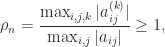
are the elements at the kth stage of Gaussian elimination. The growth factor measures how much elements grow during the elimination. We would like the product p(n)\rho_n to be of order 1, so that \Delta A is a small relative perturbation of A. We therefore need \rho_n not to be too large.

With partial pivoting, in which row interchanges are used to ensure that at each stage the pivot element is the largest in its column, Wilkinson showed that \rho_n \le 2^{n-1} and that equality is possible. Such exponential growth implies a large \Delta A (unless we are lucky), meaning a severe loss of numerical stability. However, seventy years of digital computing experience have shown that \rho_n is usually of modest size in practice. Explaining why this is the case is one of the outstanding problems in numerical analysis.

It is easy to experiment with growth factors in MATLAB. I will use the function

function g = gf(A)
%GF     Approximate growth factor.
%   g = GF(A) is an approximation to the
%   growth factor for LU factorization
%   with partial pivoting.
[~,U] = lu(A);
g = max(abs(U),[],'all')/max(abs(A),[],'all');

It computes a lower bound on the growth factor (since it only considers k=n in the numerator in the definition), but it is entirely adequate for our purposes here. Let’s compute the growth factor for a random matrix of order 10,000 with elements from the standard normal distribution (mean 0, variance 1):

>> rng(1); n = 10000; gf(randn(n))
ans =
6.1335e+01

Growth of 61 is unremarkable for a matrix of this size. Now we try a matrix of the same size generated by the gallery('randsvd') function:

>> A = gallery('randsvd',n,1e6,2,[],[],1);
>> gf(A)
ans =
9.7544e+02

This function generates an n\times n matrix with known singular value distribution and with singular vector matrices that are random orthogonal matrices from the Haar distribution. The parameter 1e6 specifies the 2-norm condition number, while the 2 (the mode parameter) specifies that there is only one small singular value, so the singular values are 1 repeated n-1 times and 1e-6. Growth of 975 is exceptional! These matrices have been in MATLAB since the 1990s, but this large growth property has apparently not been noticed before.

It turns out that mode 2 randsvd matrices generate with high probability growth factors of size at least n/(4 \log n) for any condition number and for any pivoting strategy, not just partial pivoting. One way to check this is to randomly permute the columns of
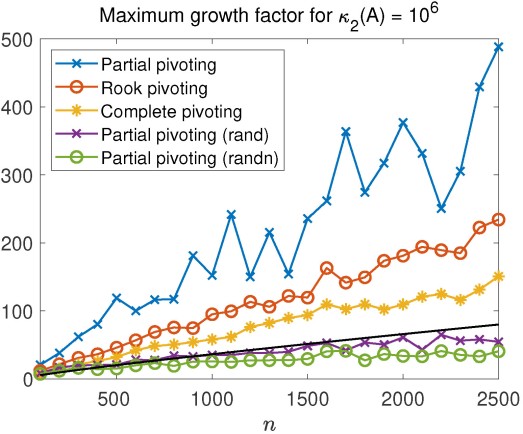
 A before doing the LU factorization with partial pivoting:

>> gf(A(:,randperm(n)))
ans =
7.8395e+02

Here is a plot showing the maximum over 12 randsvd matrices for each n of the growth factors for three different pivoting strategies, along with the maximum growth factors for partial pivoting for rand and randn matrices. The black curve is n/(4 \log n). This plot emphasizes the unusually large growth for mode 2 randsvd matrices.

growth_randsvd_max_1e6.jpg

What is the explanation for this large growth? It stems from three facts.

  • Haar distributed orthogonal matrices have the property that that their elements are fairly small with high probability, as shown by Jiang in 2005.
  • If the largest entries in magnitude of A and A^{-1} are both small, in the sense that their product is \theta \ll 1, then A will produce a growth factor of at least 1/\theta for any pivoting strategy. This was proved by Des Higham and I in the paper Large Growth Factors in Gaussian Elimination with Pivoting.
  • If W is an orthogonal matrix generating large growth then a rank-1 perturbation of 2-norm at most 1 tends to preserve the large growth.

For full details see the new EPrint Random Matrices Generating Large Growth in LU Factorization with Pivoting by Des Higham, Srikara Pranesh and me.

Is growth of order n a problem in practice? It can be for two reasons.

  • The largest dense linear systems Ax = b solved today are of dimension n = 10^7. If we work in single precision then nu \approx 1 and so LU factorization can potentially be completely unstable if there is growth of order n.
  • For IEEE half precision arithmetic growth of order n will cause overflow once n exceeds 10^5 / \max_{i,j} |a_{ij}|. It was overflow in half precision LU factorization on randsvd matrices that alerted us to the large growth.
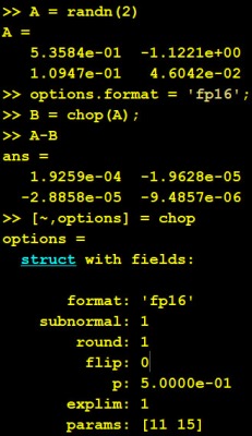
Simulating Low Precision Floating-Point Arithmetics in MATLAB

At least five floating-point arithmetics are available in mainstream hardware:

  • the IEEE double precision (fp64), single precision (fp32), and half precision (fp16) formats,
  • bfloat16, and
  • tf32, introduced in the recently announced NVIDIA A100, which uses the NVIDIA Ampere GPU architecture.

Only fp32 and fp64 are available on current Intel processors and most programming environments support only these two precisions. For many of us it is therefore necessary to simulate other precisions if we wish to explore their properties and the behavior of algorithms when run at these precisions.

chop-ex.jpg

Srikara Pranesh and I have written a MATLAB function chop that allows arithmetic of arbitrary precision and exponent range (both lower than fp64) to be simulated. The idea is very simple: variables are stored in fp32 or fp64 and then rounded to the required precision and exponent range after each operation by calling chop. The precision and range, as well as various other parameters, can be changed at any point in the computation.

Our approach can be compared with defining a new data type and storage format and converting to and from single precision or double precision in order to carry out the computations. Our approach avoids the overheads of repeatedly converting to and from the special storage format. It gains speed and generality at the cost of requiring chop calls to be inserted in the code.

Chop is available from this GitHub repository and from MathWorks File Exchange. The motivation behind chop is described in this open access paper in SIAM. J. Sci. Comput. We have made use of chop to simulate fp16 and bfloat16 in several recent papers, including on mixed precision algorithms, probabilistic rounding error analysis, and fast and accurate summation.

How to Use Chop

A call to chop has the form chop(X,options), where the structure options spceifies how to round the elements of the real array X to a lower precision arithmetic. X should be a single precision or double precision array and the output will have the same type. The structure options controls various aspects of the rounding, as we now explain.

  1. The arithmetic format is specified by options.format, which is one of
    • ‘b’, ‘bfloat16’: bfloat16,
    • ‘h’, ‘half’, ‘fp16’: IEEE half precision (the default),
    • ‘s’, ‘single’, ‘fp32’: IEEE single precision,
    • ‘d’, ‘double’, ‘fp64’: IEEE double precision,
    • ‘c’, ‘custom’: custom format.

    In the last case the (base 2) format is defined by options.params, which is a 2-vector [t,emax], where t is the number of bits in the significand (including the hidden bit) and emax is the maximum value of the exponent.

  2. options.subnormal specifies whether subnormal numbers are supported (if they are not, subnormals are flushed to zero):
    • 0 = do not support subnormals (the default for bfloat16),
    • 1 = support subnormals (the default for fp16, fp32, and fp64).
  3. The form of rounding is specified by options.round:
    • 1: round to nearest using round to even last bit to break ties (the default);
    • 2: round towards plus infinity (round up);
    • 3: round towards minus infinity (round down);
    • 4: round towards zero;
    • 5: stochastic rounding—round to the next larger or next smaller floating-point number with probability proportional to 1 minus the distance to those floating-point numbers;
    • 6: stochastic rounding—round to the next larger or next smaller floating-point number with equal probability.

    For stochastic rounding, exact floating-point numbers are not changed.

  4. If options.flip = 1 (default 0) then each element of the rounded result has, with probability options.p (default 0.5), a randomly chosen bit in its significand flipped. This option is useful for simulating soft errors.
  5. If options.explim = 0 (default 1) then emax (the maximal exponent) for the specified arithmetic is ignored, so overflow, underflow, or subnormal numbers will be produced only if necessary for the data type of X. This option is useful for exploring low precisions independent of range limitations.

To avoid repeatedly passing the options argument, one can issue a call chop([],options) and the subsequent calls will use the previously given options parameters. The value of options can be inspected with [~,options] = chop.

In the rest of this post we give examples of the use of chop.

Fp16 versus Bfloat

The code

x = 1/3;
opt_h.format = 'h'; xh = chop(x,opt_h); err_h = (x - xh)/x
opt_b.format = 'b'; xb = chop(x,opt_b); err_b = (x - xb)/x
x = 70000;
xh = chop(x,opt_h)
xb = chop(x,opt_b)

produces the output

err_h =
2.4414e-04
err_b =
-1.9531e-03
xh =
Inf
xb =
70144

which illustrates the higher precison but smaller range of fp16 compared with bfloat16.

Rounding Modes

The code

opt.format = 'h'; x = 0.1; rng(2)
for k = 1:6
opt.round = k;
y(k) = chop(x,opt);
end
errors = y - x
diff_y = diff(y)

rounds 0.1 to fp16 using six different rounding modes. The output is

errors =
-2.4414e-05   3.6621e-05  -2.4414e-05  -2.4414e-05  -2.4414e-05
3.6621e-05
diff_y =
6.1035e-05  -6.1035e-05            0            0   6.1035e-05

Rounding maps a number to the next larger or next smaller floating-point number, so there are only two possibilties for the error, and they have opposite signs. The diff_y values are consistent with the spacing of the fp16 floating-point numbers around 0.1, which is 2^{-11}/8.

Matrix Multiplication

The overheads of chop can be minimized by choosing a suitable implementation of a computation. Matrix multiplication provides a good example. The multiplication C = A*B of n-by-n matrices involves 2n^3 floating-point operations, each of which needs to be chopped. The following code uses only 2n calls to chop, because it processes an outer product in a single call, taking advantage of the fact that chop can take a matrix argument.

A = rand(m,n); B = rand(n,p);
C = zeros(m,p);
for i = 1:n
C = chop(C + chop(A(:,i)*B(i,:)));
end

Tf32 Arithmetic

The recently announced NVIDIA A100 GPU supports a new floating-point format called tf32 in its tensor cores. Tf32 is a 19-bit format that has 11 bits in the significand (including the hidden bit) and 8 bits in the exponent. So it has the precision of fp16 and the range of bfloat16, effectively combining the best features of these two formats. We can simulate tf32 using the custom format of chop. The code

opt.format = 'custom';
% tf32. Significand: 10 bits plus 1 hidden, exponent: 8 bits.
t = 11; emax = 127;
opt.params = [t,emax];
x = 1/3;
xt = chop(x,opt); err_t = (x - xt)/x
x = 70000;
xt = chop(x,opt)

produces the output

err_t =
2.4414e-04
xt =
70016

The error is the same as for fp16 but the number 70000 now rounds to a finite floating-point number.

Singular Values of Rank-1 Perturbations of an Orthogonal Matrix

What effect does a rank-1 perturbation of norm 1 to an n\times n orthogonal matrix have on the extremal singular values of the matrix? Here, and throughout this post, the norm is the 2-norm. The largest singular value of the perturbed matrix is bounded by 2, as can be seen by taking norms, so let us concentrate on the smallest singular value.

Consider first a perturbation of the identity matrix: B = I + xy^T, for unit norm x and y. The matrix B has eigenvalues 1 (repeated n-1 times) and 1 + y^Tx. The matrix is singular—and hence has a zero singular value—precisely when y^Tx = -1, which is the smallest value that the inner product y^Tx can take.

Another example is B = A + yy^T, where A = I - 2yy^T and y has unit norm, so that A is a Householder matrix. Here, B = I - yy^T is singular with null vector y, so it has a zero singular value,

Let’s take a random orthogonal matrix and perturb it with a random rank-1 matrix of unit norm. We use the following MATLAB code.

n = 100; rng(1)
A = gallery('qmult',n); % Random Haar distrib. orthogonal matrix.
x = randn(n,1); y = randn(n,1);
x = x/norm(x); y = y/norm(y);
B = A + x*y';
svd_B = svd(B);
max_svd_B = max(svd_B), min_svd_B = min(svd_B)

The output is

max_svd_B =
1.6065e+00
min_svd_B =
6.0649e-01

We started with a matrix having singular values all equal to 1 and now have a matrix with largest singular value a little larger than 1 and smallest singular value a little smaller than 1. If we keep running this code the extremal singular values of B do not change much; for example, the next run gives

max_svd_B =
1.5921e+00
min_svd_B =
5.9213e-01

A rank-1 perturbation of unit norm could make A singular, as we saw above, but our random perturbations are producing a well conditioned matrix.

What is the explanation? First, note that a rank-1 perturbation to an orthogonal matrix A can only change two of the singular values, because the singular values are the square roots of the eigenvalues of A^T A, which is the identity plus a rank-2 matrix. So n-2 singular values remain at 1.

A result of Benaych-Georges and Nadakuditi (2012) says that for large n the largest and smallest singular values of B tend to (1+\sqrt{5})/2 = 1.618\dots and (-1+\sqrt{5})/2 = 0.618\dots respectively! As our example shows, n does not have to be large for these limits to be approximations correct to roughly the first digit.

The result in question requires the original orthogonal matrix to be from the Haar distribution, and such matrices can be generated by A = gallery('qmult',n) or by the construction

[Q,R] = qr(randn(n));
Q = Q*diag(sign(diag(R)));

(See What Is a Random Orthogonal Matrix?.) The result also requires u and v to be unit-norm random vectors with independent entries from the same distribution.

However, as the next example shows, the perturbed singular values can be close to the values that the Benaych-Georges and Nadakuditi result predicts even when the conditions of the result are violated:

n = 100; rng(1)
A = gallery('orthog',n);   % Random orthogonal matrix (not Haar).
x = rand(n,1); y = (1:n)'; % Non-random y.
x = x/norm(x); y = y/norm(y);
B = A + x*y';
svd_B = svd(B);
max_svd_B = max(svd_B), min_svd_B = min(svd_B)
max_svd_B =
1.6069e+00
min_svd_B =
6.0687e-01

The question of the conditioning of a rank-1 perturbation of an orthogonal matrix arises in the recent EPrint Random Matrices Generating Large Growth in LU Factorization with Pivoting.

Update of Catalogue of Software for Matrix Functions

funm_ex.jpg

Edvin Hopkins and I have updated to version 3.0 the catalogue of software for matrix functions that we originally produced in 2014 and updated in 2016. It covers what is available in various languages (C++, Fortran, Java, Julia, Python, Rust), problem solving environments (GNU Octave, Maple, Mathematica, MATLAB and associated toolboxes, R, Scilab), and libraries (Armadillo, GNU Scientific Library, NAG Library, SLEPc, SLICOT).

Here are some highlights of changes in the last four years that are reflected in the new version.

  • Several new MATLAB third-party functions have been written, by various authors, notably for f(A)b and for arbitrary precision evaluation of the exponential and logarithm.
  • Matrix function support in Julia has been expanded.
  • Armadillo, Rust, SLEPc, and Tensorflow are included in new entries.

In addition, all URLs and references have been updated.

Suggestions for inclusion in a future revision are welcome.